Bercovier-Engelman test
The exact solution of Bercovier-ENgelman [BE79] is defined on \(\Omega=\[0, 1]^3\) by:
\[\begin{eqnarray}
u_1 &=& -256y(y-1)(2y-1)x^2(x-1)^2\\
u_2 &=& 256x(x-1)(2x-1)y^2(y-1)^2\\
u_3 &=& 0\\
p &=& (x-0.5)(y-0.5)
\end{eqnarray}\]
External forces are calculated using exact solution in the Stokes / Navier-Stokes equations.
Dirichlet conditions
We compare the approximated solution and the exact solution of Bercovier-Engelman, respectively for pressure (Figure 1 and Figure 2) and velocity (Figure 3 and Figure 4).
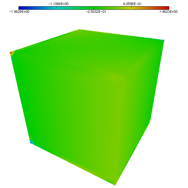
Figure 1. Pressure on the unit cube. Computed solution
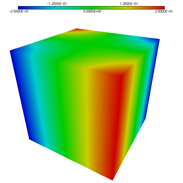
Figure 2. Pressure on the unit cube. Exact solution
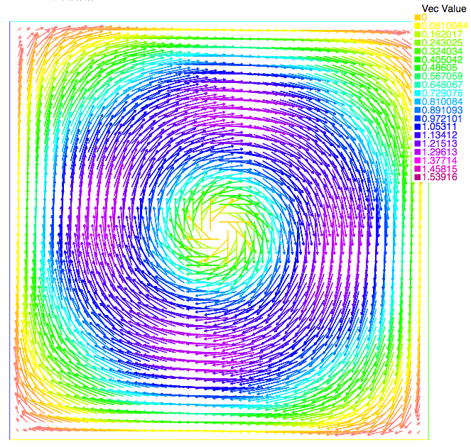
Figure 3. Velocity field on the unit cube on the cut z=0.5. Computed solution
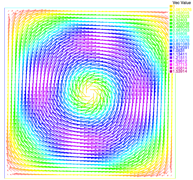
Figure 4. Velocity field on the unit cube on the cut z=0.5. Exact solution
FreeFem++ algorithm:
-
Stokes_BE_dirichlet.edp
-
Navier-Stokes_BE_dirichlet.edp
Mixed conditions
We compare the approximated solution and the exact solution of Bercovier-Engelman, respectively for pressure (Figure 5 and Figure 6) and velocity (Figure 7 and Figure 8).
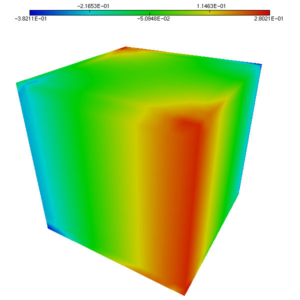
Figure 5. Pressure on the unit cube. Computed solution
Figure 6. Pressure on the unit cube. Exact solution
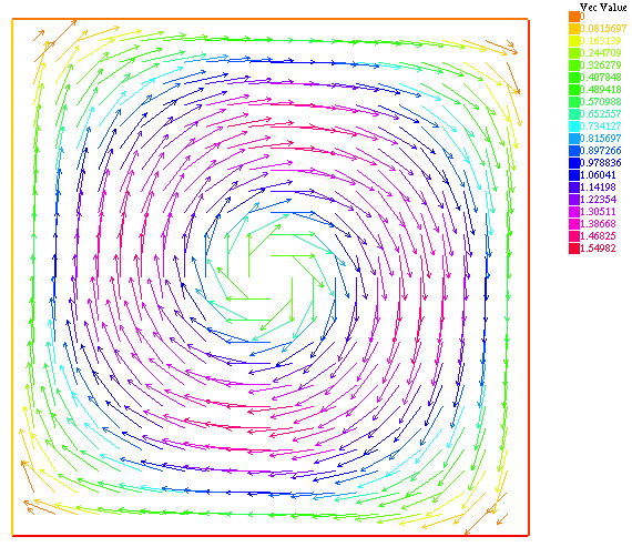
Figure 7. Velocity field on the unit cube on the cut z=0.5. Computed solution
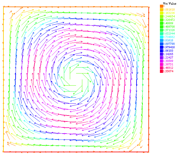
Figure 8. Velocity field on the unit cube on the cut z=0.5. Exact solution