Stokes steady case
Let \(\Omega\subset\mathbb{R}^3\) be a bounded domain with a Lipschitz-continuous boundary \(\Gamma\). Suppose that \(\Gamma\) consists of two measurable parts \(\Gamma_D\) and \(\Gamma_N\) where a Dirichlet and a Neumann condition are imposed respectively. Flows at low Reynold’s number satisfy the Stokes problem:
Where \(\mathbf{u}=(u_1, u_2, u_3)\) is the fluid velocity, \(p\) its pressure, \(\nu\) its kinematic viscosity and \(\mathbf{f}\) an applied force.
The differents operators are defined (in dimension \(N\)) by:
Variational form
We set \(V=H_0^1(\Omega)^3=\left\{v\in H^1(\Omega)^3 | v_{|\Gamma_D}=0\right\}\) and \(Q=L_0^2(\Omega)=\left\{q\in L^2(\Omega) | \int_{\Omega}{q}=0\right\}\). We then multiply the equation \(\eqref{eqstokes:1}\) by \(\mathbf{v}\in V\) and the equation \(\eqref{eqstokes:2}\) by \(q\in Q\), then integrate the equations over \(\Omega\) , it holds:
Applying the Green’s formula, we get:
Since \(\mathbf{v}\) belongs to \(V\), the variational form becomes: Find \(\mathbf{u}\in V\), \(p\in Q\) such as:
Taylor-Hood spaces
Let \(V_h\subset V\) and \(Q_h\subset Q\) be subspaces of inite dimensions such as \(V_h\rightarrow V\) and \(Q_h\rightarrow Q\) when \(h\rightarrow 0\). We consider the approximated Stokes problem:
Find \(\mathbf{u}_h\in V_h\) and \(p_h\in Q_h\) sush as:
This problem is well-defined if the spaces Vh and Qh verify the inf-sup condition:
We can note that Stokes equations only use secoind derivatives for the velocity \(u\) and first derivative for the pressure \(p\), so it makes sense to use \(k\geq 1\) polynomial degree for \(V_h\) and \(k−1\) degree for \(Q_h\). Here, we put \(k=2\).
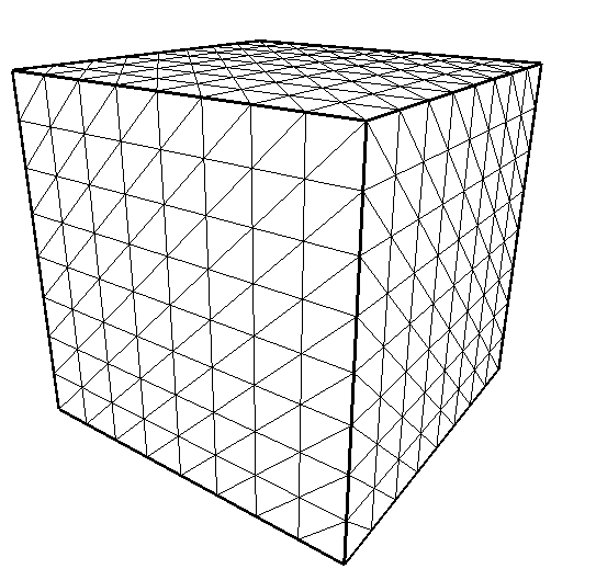
A regular triangulation \(Th\) of \(\Omega\), such as \(\bar{\Omega}=\bigcup_{K\in T_h}{K}\), verifies:
-
Each \(K\) is a polyhedron such as \(int(K)\ne 0\)
-
\(\text{int}(K_1)\cap \text{int}(K_2)=\emptyset\) for each \(K_1\) distincts to \(K_2\) .
-
if \(E=K_1\cap K_2\), then \(E\) is either a shared face, a shared edge or a share vertex.
Finally, we define the Taylor-Hood space in the following way:
where \(X_h^r = \left\{g\in \mathcal{C}(\bar{\Omega}), \forall K\in T_h, g_{|K}\in\mathbb{P}^r\right\}\)
The Taylor-Hood spaces verify the inf-sup conditions and according to [GR86] we have the convergence estimation:
FreeFem++ code
In the Dirichlet condition only case, it is necessary to fix the constant part of the pressure. We add a stabilization term to the weak form:
Where \(\epsilon\) is small, typically between \(10−6\) and \(10−10\). The following program solves the Stokes equations on a cube with a given velocity:
load "msh3"

//Mesh
int nn = 8;
mesh T2d = square(nn, nn);
mesh3 Th = buildlayers(T2d, nn, zbound=[0., 1.]);

//Parameters
real mu = 1.;

//Easy ktest
func f1 = 1.;
func f2 = 1.;
func f3 = 1.;
func uEx = x;
func vEx = y;
func wEx = -2*z;
func pEx = x+y+z-3/2.;

//Taylor Hood spaces
fespace Vh(Th,P2);
Vh u1, u2, u3;
Vh v1, v2, v3;
fespace Qh(Th, P1);
Qh p, q;

//Weak formulation
solve Stokes ([u1,u2,u3,p], [v1,v2,v3,q], solver=UMFPACK)
    = int3d(Th)(
          mu * (
              dx(u1)*dx(v1) + dy(u1)*dy(v1) + dz(u1)*dz(v1)
            + dx(u2)*dx(v2) + dy(u2)*dy(v2) + dz(u2)*dz(v2)
            + dx(u3)*dx(v3) + dy(u3)*dy(v3) + dz(u3)*dz(v3)
        )
        - p * q * 1e-10
        - p*dx(v1) - p*dy(v2) - p*dz(v3)
        - dx(u1)*q - dy(u2)*q - dz(u3)*q
    )
    - int3d(Th)(
          f1*v1 + f2*v2 + f3*v3
    )
    + on(1, 2, 3, 4, 5, 6, u1=uEx, u2=vEx, u3=wEx)
    ;

plot(p, fill=true);
Uzawa method
We have to solve the following problem:
This problem is equivalent to the matricial form:
Where A, B and F are the respectives representatives matrices of the bilinear forms:
The Uzawa [RT93] algorithm consists of minimizing the functionnal:
Under the constraint \(B=0\)
| For more information, see Uzawa method |
The Uzawa algorithm reads:
The following program solves the Stokes equations using the Uzawa method on a cube with a given velocity:
load "msh3"

//Mesh
int nn = 8;
mesh T2d = square(nn, nn);
mesh3 Th = buildlayers(T2d, nn, zbound=[0., 1.]);

//Parameters
real mu = 1.;

//Easy ktest
func f1 = 1.;
func f2 = 1.;
func f3 = 1.;
func uEx = x;
func vEx = y;
func wEx = -2*z;
func pEx = x+y+z-3/2.;

//Taylor Hood spaces
fespace Vh(Th,P2);
Vh u1, u2, u3;
fespace Qh(Th, P1);
Qh p;

//Weak formulation
macro grad(a) [dx(a), dy(a), dz(a)] //

varf vA(u, v)
    = int3d(Th)(
          mu * grad(u)' * grad(v)
    )
    + on(1, 2, 3, 4, 5, 6, u=0.)
    ;

varf vBX(q, v)
    = int3d(Th)(
          q * dx(v)
    )
    ;

varf vBY(q, v)
    = int3d(Th)(
          q * dy(v)
    )
    ;

varf vBZ(q, v)
    = int3d(Th)(
          q * dz(v)
    )
    ;

varf vOnX(u, v)
    = on(1, 2, 3, 4, 5, 6, u=uEx)
    + int3d(Th)(
        f1 * v
    )
    ;

varf vOnY(u, v)
    = on(1, 2, 3, 4, 5, 6, u=vEx)
    + int3d(Th)(
        f2 * v
    )
    ;

varf vOnZ(u, v)
    = on(1, 2, 3, 4, 5, 6, u=wEx)
    + int3d(Th)(
        f3 * v
    )
    ;

matrix A = vA(Vh, Vh, solver=sparsesolver);
matrix BX = vBX(Qh, Vh);
matrix BY = vBY(Qh, Vh);
matrix BZ = vBZ(Qh, Vh);

real[int] OnX = vOnX(0, Vh);
real[int] OnY = vOnY(0, Vh);
real[int] OnZ = vOnZ(0, Vh);

func real[int] Uzawa (real[int] &pp){
    real[int] bX = OnX; bX += BX * pp;
    real[int] bY = OnY; bY += BY * pp;
    real[int] bZ = OnZ; bZ += BZ * pp;

    u1[] = A^-1 * bX;
    u2[] = A^-1 * bY;
    u3[] = A^-1 * bZ;

    pp  = BX' * u1[];
    pp += BY' * u2[];
    pp += BZ' * u3[];
    pp  = -pp;

    return pp;
}

p=0.;
LinearCG(Uzawa, p[], eps=1.e-6);

plot(p, fill=true);