Ethier-Steinmann test

The exact solution of Ethier-Steinmann [ES94]is defined on \(\Omega=[-1,1\)^3] by:

\[\begin{eqnarray} u_1 &=& -a(a^{ax}\sin(ay+dz) + e^{az}\cos(ax+dy))\\ u_2 &=& -a(e^{ay}\sin(az+dx) + e^{ax}\cos(ay+dz))\\ u_3 &=& -a(e^{az}\sin(ax+dy) + e^{ay}\cos(az+dx))\\ p &=& \frac{-a^2}{2}(e^{2ax}+e^{2ay}+e^{2az}\\\nonumber && +2\sin(ax+dy)\cos(az+dx)e^{a(y+z)}\\\nonumber &&+ 2\sin(ay+dz)\cos(ax+dy)e^{a(x+z)}\\\nonumber &&+ 2\sin(az+dx)\cos(ay+dz)e^{a(x+y)}) \end{eqnarray}\]

With \(a=\frac{\pi}{4}\) and \(d=\frac{\pi}{2}\)

External forces are calculated using exact solution in the Stokes / Navier-Stokes equations.

Dirichlet conditions

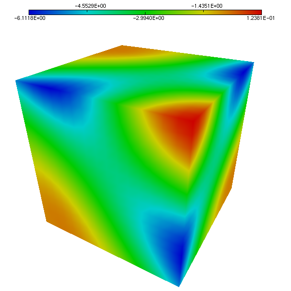
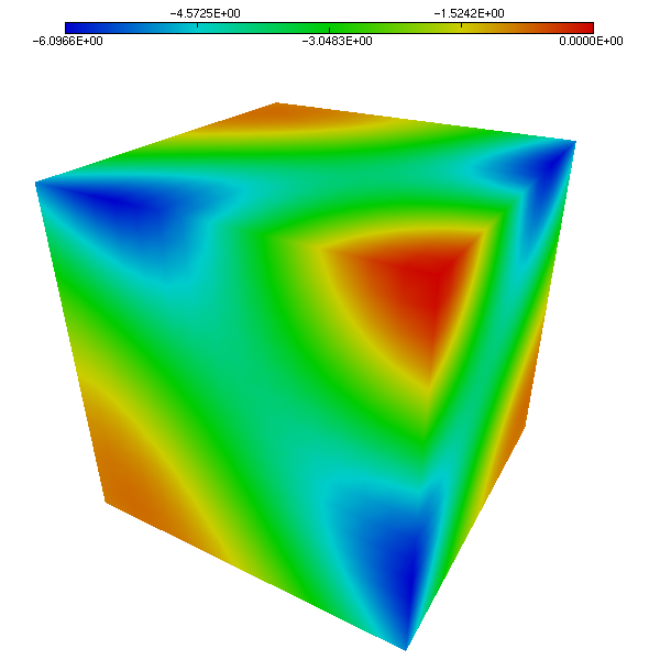
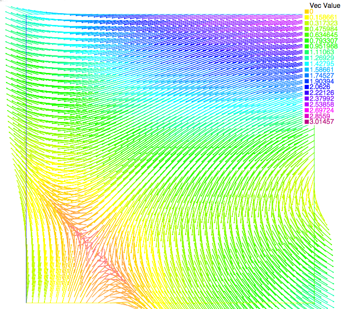
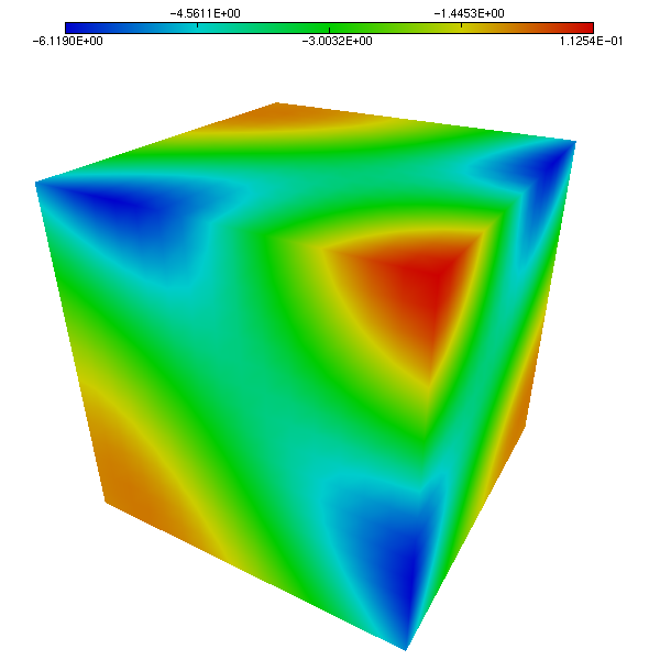
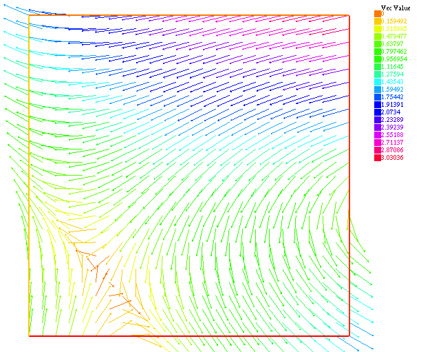
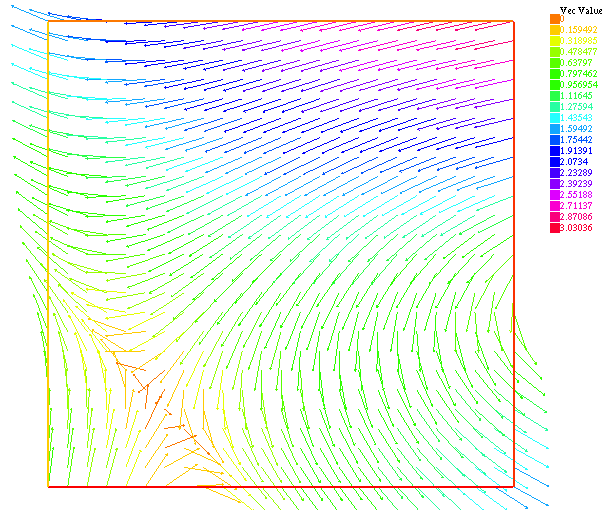
The following figures allow to compare the approximated solution and the exact solution of Etheir-Steinmann, respectively for the pressure (Figure 1 and Figure 2) and velocity (Figure 3 and Figure 4 ). Visually speaking, the approximated solutions and the exact solutions are very closed.

Figure 1. Computed solution pressure on the unit cube

Figure 2. Exact solution pressure on the unit cube

Figure 3. Computed solution velocity field on the unit cube on the cut y=-1.

Figure 4. Exact solution velocity field on the unit cube on the cut y=-1.

FreeFem++ algorithm:

Stokes_ES_dirichlet.edp
Navier-Stokes_ES_dirichlet.edp

Mixed conditions

We compare the approximated solution and the exact solution of Etheir-Steinmann, respectively for the pressure (Figure 5 and Figure 6 ) and velocity (Figure 7 and Figure 8). Visually speaking, the approximated solutions and the exact solutions are very closed.

Figure 5. Pressure on the unit cube. Computed solution

Figure 6. Pressure on the unit cube. Exact solution

Figure 7. Velocity field on the unit cube on the cut y=0. Computed solution

Figure 8. Velocity field on the unit cube on the cut y=0. Exact solution

FreeFem++ algorithm:

Stokes_ES_mixed.edp
Navier-Stokes_ES_mixed.edp